


This article is developed to help Computer Vision beginners in getting a adequate grasp of working procedure for a Image Classification problem.
Computer Vision has been widely acknowledged as one of the most important fields which is ubiquitously applied in industry or in the real life. Recently, with the advance in Machine Learning especially Deep Learning, Computer Vision has been reaching the brand new level of perceiving images, videos captured from the surrounding environments, and covering a variety of research topics including Image Classification, Object Detection to Action Recognition and so on. This article is developed to help Computer Vision beginners in getting an adequate grasp of working procedure for a Image Classification problem.
CIFAR10 dataset is utilized in training and test process to demonstrate how to approach and tackle this task. Besides, common well-known CNN architectures are used with modern Learning Rate schedule for illustrating their efficiency and gaining high accuracy level within a small number of training epochs.
Table of Contents:
1. Review and Prepare CIFAR10 dataset
2. Review modern CNN architectures
3. Setup Training system
4. Experiments and Results
1. Review and Prepare CIFAR10 dataset
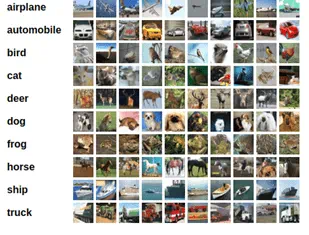
As a Computer Vision practitioner, CIFAR10 is commonly the first dataset to experience. This dataset contains 60000 32x32 color images uniformly distributed to 10 classes. Below are some samples of CIFAR10 dataset depicting 10 classes.
In the source code, this step is clearly performed in Section 2 – Prepare Data. Before applied to training or test procedure, Data Transformation are usually used to pre-process data to some standard with the purpose to optimally increase the precision of both processes. In the notebook, the author only transformed image data by a few common transforming technique e.g. Random Crop, Horizontal Flipping, and Normalization by the mean and standard deviation of CIFAR10 dataset.
(source:https://www.cs.toronto.edu/~kriz/cifar.html)
2. Review Modern CNN Architectures
In this section, it is assumed that the readers have already gained prerequisites of Deep Learning about Convolutional Neural Network layers, and implemented a basic CNN models. At the time of writing this blog, there are a significant number of CNN models serving a numerous Computer Vision topics and each model has its own strength and robustness for specific classes of applications.
To review the common CNN architectures with enough depth of knowledge, but not affect the main purpose of this blog, the author only introduce and also explain several famous architectures which shape the modern Deep Learning success.
2.1 VGG network
VGGNet is the 1st runner-up in ILSVRC 2014 in the classification task. It is the first network that uses block as unit component. Each block consists of a series of convolutional layers, followed by a max pooling layer for spatial downsampling. The authors of VGGNet used 3x3 kernels for convolution. Later on, inherited their ideas, VGGNet is customized to use 5x5, 7x7 kernels for specific situations. All common VGG models are depicted below:

(source: https://medium.com/coinmonks/paper-review-of-vggnet-1st-runner-up-of-ilsvlc-2014-image-classification-d02355543a11) VGGNet imlementation can be found here [link]
2.2 ResNet network

(soruce: https://towardsdatascience.com/review-resnet-winner-of-ilsvrc-2015-image-classification-localization-detection-e39402bfa5d8) ResNet implementation from scratch are shown here [link]
ResNet is the most ubiquitous network that can be applied in many application and its efficiency is clearly proved after the winning at ILSVRC 2015. ResNet follows VGG’s 3x3 convolutional layer design and it introduces the residual block with the additional Identity mapping by Shortcuts. The residual blocks not only help increase the function complexity but also reduce the training errors.
2.3 Inception network
The last network covered in this blog is Inception, which achieved 1st runner up in Image Classification task in ILSVRC 2015. There are 4 version of Inception networks at this time, the first one is GoogleNet. Inception block consists of 4 parallel paths with different components. Their connections performed convolution with different kernel sizes of 1x1, 3x3 and 5x5. Their ouputs are concatenated along the channel dimensions to comprise the block’s output. Inception block are illustrated in the following figure:

(source: https://arxiv.org/pdf/1409.4842.pdf)
(Read more: Text Summarization in Machine Learning)
3. Setup Training system
After preparing dataset and defining network model, the next step is to setup the training system. To be more specific, we need to define Loss function, Optimizer and some other Hyper-parameters that support the training procedure.
3.1 Loss function
Loss function is the component of the training system quantifying the badness of the model. The choice of Loss function depends heavily on the the problem type. For numerical values, the most common cost functions is Square Error. For classification task, Cross-Entropy is commonly preferred. In this dataset, there are 10 classes, the proper loss function is clearly the Cross-Entropy loss. Softmax operation is also applied to map the result to range [0, 1] as related to probability. Formula for the chosen loss function is defined below:
p = softmax(pred)
L = -∑ log(pi, label I)
3.2 Optimizer
After calculating the current loss of training’s specific state, a mechanism is needed to search and update the parameters for minimizing the loss value. As widely known, the most popular optimization algorithm for Neural Networks is Gradient Descent. Briefly, at a state, for each parameter, the optimizer will determined how to change its value to reach the lowest minima for the cost function.
There are also numerous options for optimizer e.g. Stochastic Gradient Descent, Adam, RMSProp , … In this work, we will utilize SGD optimizer. Reader can conduct more experiments with other algorithms as mentioned.
3.3 Learning Rate schedule
Define the value of Learning Rate for Stochastic Gradient Descent algorithm is significantly important due to its control of the speed of convergence and the performance of trained networks. Depending on the state of training model, the learning rate should be adjusted to minimize the loss value. LR schedule is still the active field for research. In this blog, the author introduce the state-of-the-art LR schedule which efficiently change LR values and rapidly obtain high accuracy that is 1-Cycle scheduler. We use a single and symmetric cycle of the triangular schedule, then perform a cool-down schedule. In my work, 1-Cycle is setup as the following:

In the above figure, LR is initialized with 0.008 and continuously increase to 0.12, then decrease to 0.008 again, this process undergoes 40 epochs. In the last 10 epochs, LR is gradually reduced to 0.0008 as the final value.
4. Experiments and Results
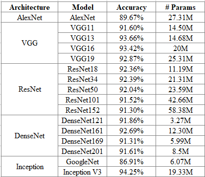
To tackle the CIFAR10 dataset, multiple CNN models are experimented to compare the different in both accuracy, speed and the number of parameters between these architectures.
Only 50 epochs are trained for each model. Actually, the LR schedule is set with distinct set of value and those values are obtained by performing LR range test as guided from the original paper.
The below table show the test accuracy after training each networks:
Several Training histories are shown below:

From the training history figure, we can see the accuracy curves are still getting higher. Due to the purpose of proving the effect of 1-Cycle schedule, so the author just trained with 50 epochs. Readers can conduct experiments with larger number of epochs and other LR schedule to obtain higher accuracy.
Interested in other technology blogs? Click here for more!
Reference
- Repository of this blog [link]
- Super-Convergence: Very Fast Training of Neural Networks Using Large Learning Rates [link]
- Diving into Deep Learning [link]
- Very Deep Convolutional Networks for Large-scale Image Recognition [link]
- Deep Residual Learning for Image Recognition [link]
- Going Deeper with Convolutions [link]


